Charting Time over Time in Splunk
In the business world, people are looking at ways to constantly improve processes and systems. The only way to determine if progress is being made is to compare performance over a period of time to that same period of time a day ago, a week ago, a month ago, or even longer.
Since Splunk gives companies the ability to store and search data over a variety of time periods, this should be an easy task to do, right?
Not so fast…
While Splunk is driven by time, the answer is a little more complex than that.
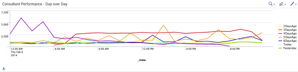
Let’s say for example that you would like to chart the same data comparing the last 6 days and today. In order to chart one time period over another time period, the search would have to disguise each day’s time to appear as if it’s today. The reason for this is so when you plot the lines on the same time chart, you can easily spot the variations across the days. Since Splunk is an expert at detecting time, this disguise is rather complex!
Before we discuss our master plan of disguise, here are some things we need to first consider:
- What time periods do I want to compare?
- How can I convince Splunk that these time periods are the same?
- How can I plot this in a dashboard that is beneficial to users?
In this example, we are going to compare the last 7 days of data by the hour with today’s data. We will use the eval command to convert time to look like today’s time and then we will use the timechart to show the different days by hour.
Note: This search will be heavy, be sure to make the search as specific as possible before the first pipe!
The first thing we need to add is a benchmark search. We will remove this search at the end, but it serves to provide each hour with data. This is very important if you are using dropdowns with values that might vary from day to day.
The search for the Benchmark is as follows:
index=star sourcetype=syslog vendor=function1 consultant=* earliest=-1d@d latest=-0d@d|eval _time=_time+86400 | timechart span=1h count | rename count AS Benchmark
This search establishes the hourly time chart to allow for the join command to execute effectively. We use yesterday’s time as opposed to today’s time as a benchmark so that all of the hours are populated with data and present in the results. We have to use the eval command to disguise time from Yesterday to Today.
eval _time=_time+86400
By using the eval command, the benchmark time chart reflects the hours from today. Off to a good start!
Next we will start to add the day over day compares. Let’s start with yesterday…
Yesterday will begin with a join command to join its search to the benchmark results by hour.
| join type=outer _time
The next piece of the search is the same as the benchmark search except consultant will be a variable $consultant$. This will give the user the ability to select a specific consultant to evaluate performance from day to day. The earliest and latest time restricts the search to Yesterday.
index=star sourcetype=syslog vendor=function1 consultant=$consultant$ earliest=-1d@d latest=-0d@d
We use the eval command to “disguise” Yesterday’s time as Today’s time. By adding 86,400 seconds to the time, Splunk thinks that Yesterday’s time is today!
|eval _time=_time+86400
Next we use the timechart command with a span of 1h, which is the same span as the Benchmark search. This is important as we are joining the searches based on the _time.
| timechart span=1h count | where count > 0 | rename count AS Yesterday]
We add the where command after the timechart to ensure that no time is plotted outside of today’s hourly range.
Rename count to yesterday to identify the line in the timechart from the other days.
Apply the same logic for the rest of the day’s you wish to plot!
Your search should look something like this:
index=star sourcetype=syslog vendor=function1 consultant=* earliest=-1d@d latest=-0d@d |eval _time=_time+86400 | timechart span=1h count | rename count AS Benchmark| join type=outer _time [search index=star sourcetype=syslog vendor=function1 consultant=$consultant$ earliest=-1d@d latest=-0d@d |eval _time=_time+86400 | timechart span=1h count | where count > 0 | rename count AS Yesterday] | join type=outer _time [search index=star sourcetype=syslog vendor=function1 consultant=$consultant$ earliest=-3d@d latest=-2d@d |eval _time=_time+(86400*3) | timechart span=1h count | where count > 0 | rename count AS 3DaysAgo ] | join type=outer _time [search index=star sourcetype=syslog vendor=function1 consultant=$consultant$ earliest=-4d@d latest=-3d@d |eval _time=_time+(86400*4) | timechart span=1h count | where count > 0 | rename count AS 4DaysAgo ] | join type=outer _time [search index=star sourcetype=syslog vendor=function1 consultant=$consultant$ earliest=-6d@d latest=-5d@d |eval _time=_time+(86400*6) | timechart span=1h count | where count > 0 | rename count AS 6DaysAgo ]| join type=outer _time [search index=star sourcetype=syslog vendor=function1 consultant=$consultant$ earliest=-5d@d latest=-4d@d |eval _time=_time+(86400*5) | timechart span=1h count | where count > 0 | rename count AS 5DaysAgo ]| join type=outer _time [search index=star sourcetype=syslog vendor=function1 consultant=$consultant$ earliest=-2d@d latest=-1d@d |eval _time=_time+(86400*2) | timechart span=1h count | where count > 0 | rename count AS 2DaysAgo ] | join type=outer _time [search index=star sourcetype=syslog vendor=function1 consultant=$consultant$ earliest=-0d@d latest=now | timechart span=1h count AS Today]| fields - Benchmark _timediff
Remember to remove the Benchmark and _timediff fields at the end!
Happy Splunking!
- Log in to post comments